Math 7
A mathematical study to the rate of change dY/dX per change of arc length dS for a given function F(X).
see the next link for the original document:
Abstract:
Most people in science are familiar with derivatives that is dY/dX. Any graph however also knows length; the arc length S. So far it is not known, to authors knowledge, however as to how this derivative behaves with respect to the distance such a graph travels, that is (dY/dX) / dS. This paper tries to solve that quest for information and discovery.
Keywords: derivative, derivative per unit of length. dY/dX, dS.
Introduction:
It is pretty straight forward: it is just a matter of creating some known graphs and see how they behave with respect to (dY/dX) / dS and see if there are some nice things to be seen. To be honest this kind of question is not known to me that does not mean there was no one in history who thought of this idea sooner than the author wanted to find out but it was simply not known. So if some-one done this before then at least for the author of this paper it is a new discovery. And if more people are unfamiliar with this type of approach of graphs; welcome to the club.
Lets get started:
To begin with investigated were some simple mathematical relationships below is a list of mathematical relationships that are currently under study:
function
F(x) = Y = X F’(X) =Y’= 1 FS’(X) = YS’ = 1 FS”(X) = YS” = see graphs
F(x) = Y = X2 F’(X) =Y’ = 2X FS’(X) = YS’ = see graphs FS”(X) = YS” = see graphs
F(x) = Y = X3 F’(X) =Y’ = 3X^2 FS’(X) = YS’ = see graphs FS”(X) = YS” = see graphs
F(x) = Y = Sin (X) F’(X) =Y’ =Cos (X) FS’(X) = YS’= see graphs FS”(X) = YS” = see graphs
F(x) = Y = (Sin (X))^2 F’(X) = Y’ = see graph FS’(X) = YS’= see graphs FS”(X) = YS” = see graphs
F(x) = Y = A*Exp(-(X-B)2) F’(X) = Y’= see graphs FS’(X) = YS’= see graphs FS”(X) = YS” = see graphs
For investigating this all the program of excel was used and in these examples dX = 0,001. One of the first things encountered is that dividing by dS, which is a small number, we encounter a great number of the end result and logically the smaller dS will be, the larger the end result will be. So to counter that the resulting function must be renormalized. This is done by the factor, the number that is encountered when X = 0. This FS’(0) is our renormalisation factor. In case of dX= 0,001 this factor is numerically 707,106722260978.
For other dX this may be a different number. If this numerical renormalisation is not done this whole exercise will blow up to infinities. Which makes sense with dS getting smaller and smaller over dX getting smaller and smaller. In 1 case the dX was lowered to 0,0001 and indeed the renormalisation a factor increased by exactly 0,001 / 0,0001 = 10 times.
The used formula to calculate dS is:
dS = square root ((dX)2 + (dY)2) = ( (dX)2 + (dY)2) 1)
This is the most common formula to calculate the distance between 2 points on a graph. Integrating this over the whole graph inbetween X1 and X2, would lead to the length of the graph arc inbetween the points of integration on the X line.
So basically what the whole study is about is the next formula:
Take any function F(x) and perform the next actions upon it;
1 (F(X2) – F(X1)) / (X2-X1) 1 (Y2 – Y1) / (X2-X1) 1 dY/dX
G(X) = ------- * -------------------------------- = ----- * -------------------------------- = ---- * ---------- = 2)
F(X0) SQRT((X2-X1)2 + (Y2-Y1)2) Y0 SQRT((X2-X1)2 + (Y2-Y1)2) Y0 dS
(dY/dX) / (Y0*dS) = (dY)/ (Y0*dX * dS) 3)
In other words it is the rate of slope change per arclength of the graph. The measure of change per unit of arc length.
Surpricingly this gave some nice unexpected results. Based on that even the derivative towards X was created .
So that also:
((dY/dX) / (Y0*dS)) / dX 4)
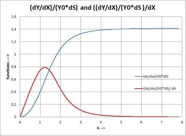
Was investigated. The easiest way to show that is graphically: F(X) = 0,1*X2 gives:
Figure 1: graphical depicting (dY/dX) / (Y0*dS) (blue) and ((dY/dX) / (Y0*dS)) / dX (red) for Y = 0,1*X2.

This is a first indication that exponential (e based) characteristics are hiding in polynomial related functions X2, X3 etc.
F(X) = 0,1* X3 gives us:
Figure 2: graphical depicting (dY/dX) / (Y0*dS) (blue) and ((dY/dX) / (Y0*dS)) / dX (red) for Y = 0,1*X3.

Also here we clearly can see that exponential (e based) characteristics are hidden in polynomial based functions and thus a confirmation of this behaviour.
F(X)= sin(X) gives us:
Figure 3: graphical depicting (dY/dX) / (Y0*dS) (blue) and ((dY/dX) / (Y0*dS)) / dX (red) for Y = sin(X).

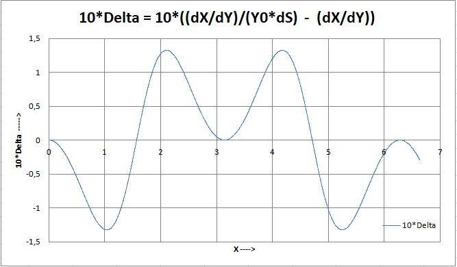
It may seem that F’(X) = cos(X) and its arc-length derivative are the same if they are not in the same graphical representation, but there is a difference. As can be shown in the next graphs:
Figure 4: F(X), F’(X) and FS’(X) for sin(X), note the difference between F’(X) and FS’(X) green vs red graph.

But there is a difference as can be seen from the next graph where the (enlarged) difference is represented:
Figure 5: difference between dy/dx and (dy/dx) /(Y0*dS)

F(X)= (sin(X))2 gives us:
Figure 6: graphical depicting (dY/dX) / (Y0*dS) (red) and ((dY/dX) / (Y0*dS)) / dX (green) for Y = (sin(X))2 (blue).

And the difference:
Figure 7: difference between dy/dx and (dy/dx) /(Y0*dS) in case of F(X) = (sin(X))2.

And for F(X) = 10*Exp(- (X - 3,5)2):
Figure 8: F(X) = 10*Exp(- (X - 3,5)2) (blue) dy/dx (red) and (dy/dx) /(Y0*dS) (green).

Figure 9: (dy/dx) /(Y0*dS) and ((dy/dx) /(Y0*dS))/dX in case of F(X) = 10*Exp(- (X - 3,5)2).

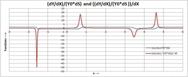
For the function F(X) = 0,1*(X - 5)*(X - 4)*(X - 3)*(X + 1)*(X + 2).
Figure: 10: F(X)= 0,1*(X - 5)*(X - 4)*(X - 3)*(X + 1)*(X + 2), F’(X) en FS’.

Figure 11: (dY/dX)/(Y0*dS) and ((dY/dX)/(Y0*dS))/dX derived from F(X)= 0,1*(X-5)*(X-4)*(X-3)*(X+1)*(X+2).

All these calculations deliver nice but graphically unexpected, at least for author, relationships.
Conclusion and discussion:
What we see is that taking the derivative as function to the arc length delivers unexpected and surprising graphs that we only know from other approaches in the mathematical world. For example that polynomial parts like X2 and X3 can be brought back to exponential relationships with a base e (Eulers number). This is confirmed in the real 5th power polynomial as is shown. Where Gaussian curve like peaks appear.
There is how ever still much to discover since these examples only represent a beginning, at least for me, of this mathematical exploration in this, for me new approach.
Acknowledgement:
The only Person I like to thank for this knowledge is God-Jesus Christ-Holy Spirit Almighty. He is the provider of all knowledge and He gave me this knowledge to pass it on to humanity. This may be not a usual way of doing in the (secular) science community, but none the less I remain with this statement. Since July 2004 I am a creationistic, Zionistic, messianic type of Christian and in my opinion God should get the honour of scientific findings on every level. Finally I like to thank my father and his girlfriend, for their support towards me amongst many other things also with respect in these findings.
References:
1]
2]
Copyright © 2022 Edgar G.J.J. Korteweg, This article is distributed under the Creative Commons Attribution License, which permits unrestricted use, distribution, and reproduction in any medium, provided the original work is properly cited. CC BY-NC-SA 4.0
Maak jouw eigen website met JouwWeb